
How Plant-Wide Energy Consumption Benchmarking Finds Waste
ISO 50006 baselines link utility use to output for ESOS-ready evidence
ESOS Phase 4 requires qualifying organisations to identify areas accounting for at least 95% of total energy consumption, yet a plant-level utility bill cannot show which line, shift or operating condition created that demand. Plant-wide energy consumption benchmarking closes this gap by comparing measured utility use with production activity under equivalent conditions.
This distinction matters commercially. A factory may consume more electricity after raising output while using less energy per tonne. Another may report a lower monthly bill because production fell, even though idle equipment and fixed loads pushed unit costs upwards.
Plant-wide energy consumption benchmarking gives energy managers a consistent reference for separating those cases. It converts electricity, gas, steam, compressed air, oil and water data into production-linked evidence such as energy per batch, cost per tonne and consumption during non-production hours. That evidence helps operations directors locate waste, prioritise investment and verify the result after work is complete.
What does plant-wide energy consumption benchmarking reveal?
A plant-wide benchmark describes expected utility consumption for a defined boundary and set of operating conditions. Actual performance can then be compared with that reference at site, department, line or equipment level.
Total consumption and energy intensity answer different questions
Total consumption shows the scale of energy purchased or generated. Energy intensity relates that consumption to an activity such as tonnes produced, batches completed or operating hours.
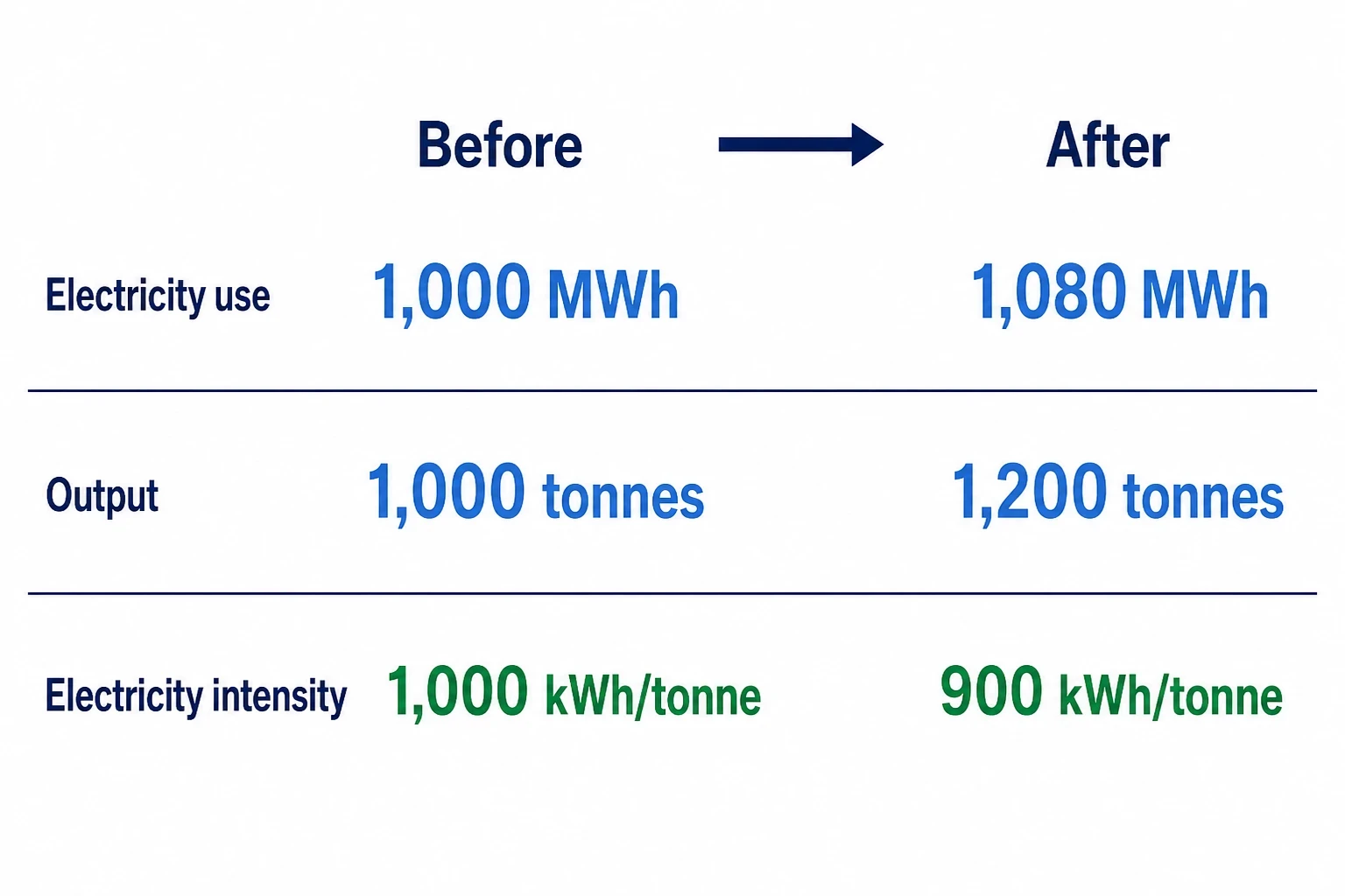
Consider a plant whose electricity use rises from 1,000 MWh to 1,080 MWh while output increases from 1,000 tonnes to 1,200 tonnes. Total electricity consumption has risen by 8%, but electricity intensity has fallen from 1,000 kWh per tonne to 900 kWh per tonne. The site has improved its production-linked performance despite using more electricity overall.
The reverse can also occur. Falling production may reduce total consumption while fixed loads remain largely unchanged. Unit energy cost then increases because the baseload is spread across fewer saleable units.
Energy managers therefore need several connected measures:
| Benchmark | Management question | Typical application |
|---|---|---|
| Total consumption | How much utility did the plant use? | Purchasing, reconciliation and reporting |
| Energy per unit of output | How efficiently did production use energy? | Line and product comparison |
| Cost per unit of output | How did energy affect manufacturing cost? | Margin analysis and investment approval |
| Non-production consumption | What remained energised without output? | Shutdown investigations |
| Peak demand | Which operating combinations created the highest load? | Demand management and capacity planning |
| Expected versus actual consumption | Did the plant use more energy than operating conditions explain? | Fault and performance-deterioration detection |
Operating-state benchmarks expose idle consumption
A single daily figure combines production, cleaning, warm standby, maintenance and shutdown periods. Separating those states produces more useful benchmarks.
An energy team can calculate typical consumption for:
- Normal production at defined throughput bands
- Start-up and heat-up periods
- Product changeovers
- Cleaning or sterilisation cycles
- Planned breaks
- Warm standby
- Full shutdown
For example, a continuous 100 kW load operating for 8,000 hours consumes 800 MWh. Part of that load may support essential refrigeration, ventilation or safety systems. The remainder may come from pumps, conveyors, extraction equipment or compressors left running between shifts.
The benchmark should use comparable non-production intervals, such as median demand during scheduled shutdown hours over an agreed baseline period. Engineers can then investigate an upward change in that interval benchmark without confusing it with increased throughput.
Omni Vision delivers turnkey utility metering, CO2 tracking, and AI-powered production KPI intelligence — giving you real-time dashboards and actionable insights across your entire facility.
How ISO 50006:2023 strengthens energy baselines
The current edition of the relevant standard is ISO 50006:2023. It provides guidance on establishing, using and maintaining energy performance indicators, known as EnPIs, and energy baselines, known as EnBs. It superseded ISO 50006:2014.
ISO 50006:2023 treats an energy baseline as a reference for evaluating performance. Normalisation allows comparison under equivalent conditions by accounting for variables that routinely and materially affect energy consumption.
Define the benchmarking boundary first
A useful hierarchy normally begins at the incoming supply and divides consumption into significant uses:
- Site utility supply
- Department or production area
- Major utility system
- Production line or process
- Selected energy-intensive equipment
The appropriate depth depends on the decision. A main electricity meter may support company reporting, but it cannot distinguish refrigeration demand from packaging demand. A compressor sub-meter can quantify compressor electricity but cannot identify which production area consumed the air unless flow measurement or another allocation method is available.
Metering should resolve a specific question. Installing a meter without defining its boundary, associated production variable and expected decision can create more data without improving the business case.
Avoid double-counting generated utilities
Plant-wide totals require careful treatment of utilities generated on site. Compressor electricity already appears within the site electricity supply. Adding an energy equivalent for delivered compressed air to the same plant total would count part of the input twice.
The same principle applies to steam raised in an on-site boiler. Fuel belongs in the site energy total. Steam measurements allocate that input to departments and processes, subject to generation and distribution losses. Purchased steam, by contrast, enters through the site boundary as an imported energy supply.
Water should normally remain a separate resource benchmark unless the analysis specifically concerns the energy required to pump, heat, cool or treat it. Maintaining this distinction preserves both the site energy balance and utility cost allocation.
Select relevant production variables
Production volume is often the dominant variable, but it may not explain consumption on its own. Appropriate variables can include:
- Product grade, recipe or format
- Good output rather than gross output
- Batch size and batch duration
- Operating hours
- Number of starts and shutdowns
- Cleaning or sterilisation cycles
- Ambient temperature
- Refrigeration or process temperature
- Rejects and rework
- Number of active lines
Static factors also need control. These are conditions that materially affect energy performance but do not change routinely, such as installed equipment, building size, line configuration or the number of shifts. A new production line or major process modification may require a baseline adjustment or a new baseline period.
Choose ratios or statistical models carefully
A ratio such as kWh per tonne is transparent and easy to communicate. It works best when output has a stable relationship with energy use and fixed consumption is small.
Ratios can mislead where a plant carries a substantial baseload. Increasing output then spreads that fixed consumption across more tonnes, causing kWh per tonne to improve even if equipment efficiency remains unchanged.
A regression model provides a stronger benchmark when several variables affect consumption. The model estimates expected energy use from factors such as throughput, product mix, operating time and temperature. Actual consumption can then be compared with the estimate for the same conditions.
The model should use energy and production data covering identical time intervals. Engineers should investigate missing readings, meter resets, shutdowns and other outliers before excluding them. Removing inconvenient observations without a documented reason can bias the baseline.
How benchmarking calculations locate energy waste
Plant-wide energy consumption benchmarking identifies waste through measurable departures from expected performance. The calculation must show what “expected” means and when a deviation warrants investigation.
Non-production baselines find avoidable running hours
For scheduled shutdown periods, analysts can group intervals by operating state and calculate typical electricity, gas, steam or compressed-air demand for each group. A persistent increase from the established shutdown benchmark indicates additional equipment use or deterioration.
The investigation can then move from the site level to the relevant sub-meter. Likely causes include:
- Fans, pumps or conveyors running through breaks
- Heating systems starting earlier than required
- Steam valves passing during shutdown
- Compressors maintaining pressure against leakage
- Refrigeration plant serving unused space
- Cleaning systems using longer cycles than the validated requirement
The benchmark identifies the affected period and utility. Maintenance and operations teams still need to confirm the physical cause.
Regression residuals expose unexplained consumption
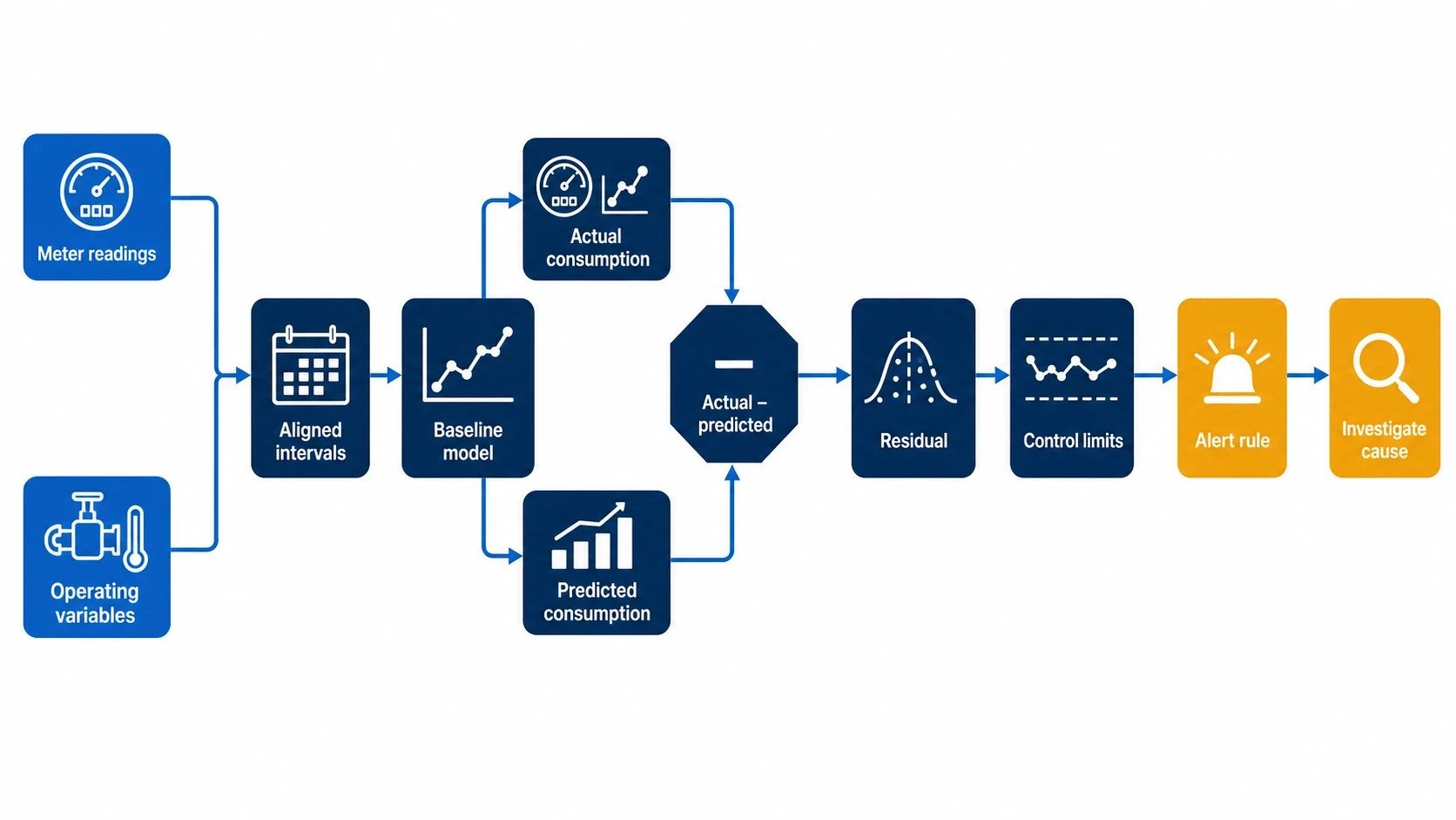
A regression-based benchmark predicts consumption for the recorded operating conditions. The difference between actual and predicted consumption is called the residual.
A positive residual means the plant used more energy than the model expected. A single large residual may reflect a data error, unusual batch or unrecorded operating event. A sequence of positive residuals can indicate sustained deterioration.
A practical alert method has four defined elements:
- A baseline model built from a representative operating period
- Relevant variables aligned to the same intervals as the meter readings
- Statistical control limits derived from the model’s normal residual variation
- An alert rule covering the size and persistence of a deviation
Control limits describe the range expected from normal process variation. An alert threshold can flag a residual outside that range or a run of smaller residuals on the same side of the expected value. The site should document the threshold, persistence rule and escalation owner. This converts anomaly detection into an auditable calculation.
Cross-utility comparisons narrow the cause
Several utility benchmarks can point to the same operational issue. Rising compressor electricity combined with stable air demand suggests poorer compressor performance or control. Rising air demand at unchanged output directs attention to leakage or additional use.
Higher boiler fuel consumption with stable steam delivery suggests a generation-efficiency problem. Stable fuel use combined with lower measured steam delivery may instead indicate a metering issue or distribution loss.
These comparisons work only when meter boundaries and timestamps align. Daily steam data compared with monthly production totals will obscure short-duration events and shift-level differences.
Building the cost-benefit case for benchmarking
The financial benefit of benchmarking comes from better project selection, earlier detection and credible savings verification. The cost includes metering, installation, commissioning, data validation, analytical work and the operating time required to investigate alerts.
Convert deviations into avoidable cost
A consumption deviation becomes financially useful when the calculation identifies:
- The affected utility
- The duration and recurrence of the deviation
- The applicable energy or water tariff
- Any demand or capacity cost
- The production conditions during the event
- The portion that engineers consider technically avoidable
Using the marginal tariff for the affected period is usually more informative than applying an annual average price. An electricity reduction during a demand peak may carry different value from the same kWh reduction overnight. Gas, water and effluent charges can also have separate volumetric and capacity components.
The calculation should keep energy savings and price effects separate. A cheaper contract lowers cost without improving plant efficiency. A production-normalised reduction in kWh, tonnes of steam or m³ of compressed air provides the technical evidence.
Rank actions by value, certainty and disruption
A project register can connect each benchmark deviation to an engineering action and financial decision:
| Opportunity type | Evidence required | Typical cost | Investment test |
|---|---|---|---|
| Scheduling correction | Non-production load profile and operating log | Low | Recurring avoidable cost versus staff time |
| Maintenance repair | Trend, inspection and post-repair measurement | Low to moderate | Repair cost versus verified annual saving |
| Control modification | Interval demand, setpoints and operating sequence | Moderate | Saving, production risk and commissioning cost |
| Equipment replacement | Normalised baseline and equipment duty profile | High | Life-cycle cost, downtime and uncertainty |
| Heat recovery | Source and sink profiles measured over representative operation | High | Annual useful heat, integration cost and production compatibility |
Simple payback can screen low-risk measures. Larger projects benefit from life-cycle cost analysis that includes maintenance, asset life, planned downtime and energy-price assumptions.
Benchmarking also exposes opportunities that should not proceed. A measured loss may be too intermittent, too small or too closely tied to production constraints to justify intervention. Rejecting a weak proposal before capital approval is part of the financial return.
Prevent double-counting between projects
A boiler optimisation project, steam-trap programme and heat-recovery installation may affect the same gas meter. Claiming each project’s estimated saving against the full site reduction can overstate the combined result.
The project register should define the measurement boundary, implementation date and interactions before work starts. Where measures overlap, teams can isolate equipment, sequence the projects or verify the combined programme at a wider boundary.
This discipline gives finance teams a traceable route from meter reading to approved saving. It also removes the unsupported assumption that an energy analytics deployment will produce a fixed percentage reduction across dissimilar plants. Savings depend on the measured opportunity, operating response and persistence of the change.
Track energy consumption, emissions, and process parameters with seamless PLC/SCADA integration via Modbus, OPC-UA, and MQTT protocols.
Using IPMVP to verify plant energy savings
IPMVP Core Concepts 2022, maintained by the Efficiency Valuation Organisation, provides a recognised framework for Measurement and Verification. IPMVP starts from a central limitation: energy savings represent avoided consumption and therefore cannot be measured directly. Analysts compare measured reporting-period consumption with an adjusted baseline representing what the plant would probably have used without the intervention.
Select a measurement boundary that fits the project
IPMVP describes four broad options:
| IPMVP option | Measurement approach | Industrial application |
|---|---|---|
| Option A | Retrofit isolation with key parameters measured | A defined equipment change where selected operating factors can be documented |
| Option B | Retrofit isolation with all relevant parameters measured | Compressor, boiler, pump or production-system projects with suitable metering |
| Option C | Whole-facility measurement | A programme containing several interacting measures |
| Option D | Calibrated simulation | Projects where measured baseline data alone cannot represent the required comparison |
Option B can provide clear attribution for an isolated system. Option C captures the combined effect of several measures, but unexplained variation across the facility can conceal smaller savings. The selection should reflect project size, expected saving, available meters and required certainty.
Write the M&V plan before implementation
The M&V plan should define:
- Baseline and reporting periods
- Metering boundary and data frequency
- Production and operating variables
- Routine adjustments for variables such as output or temperature
- Treatment of non-routine changes such as new lines or altered shift patterns
- Data-quality and missing-data procedures
- Calculation method and uncertainty
- Reporting responsibilities
For a compressed-air project, the plan may include compressor electricity, delivered airflow, system pressure, operating hours and production output. A boiler project may require fuel, steam output, return conditions, operating time and throughput.
Agreeing these details after installation creates scope for selective baselines and disputed adjustments. Pre-project agreement makes the resulting saving more credible to finance teams, auditors and board-level reviewers.
How benchmarking supports ESOS Phase 4 evidence
The Environment Agency published detailed ESOS Phase 4 guidance on 30 July 2026. Qualifying organisations must calculate total energy consumption over a 12-month reference period, using a full year of verifiable data where reasonably practicable. They must also calculate at least one energy intensity ratio for industrial processes where that category uses energy.
For industrial processes, the guidance recommends relating process energy consumption in kWh to total industrial output. Separate ratios may be appropriate where products use different units or have materially different processing requirements.
Phase 4 requires evidence of achieved savings
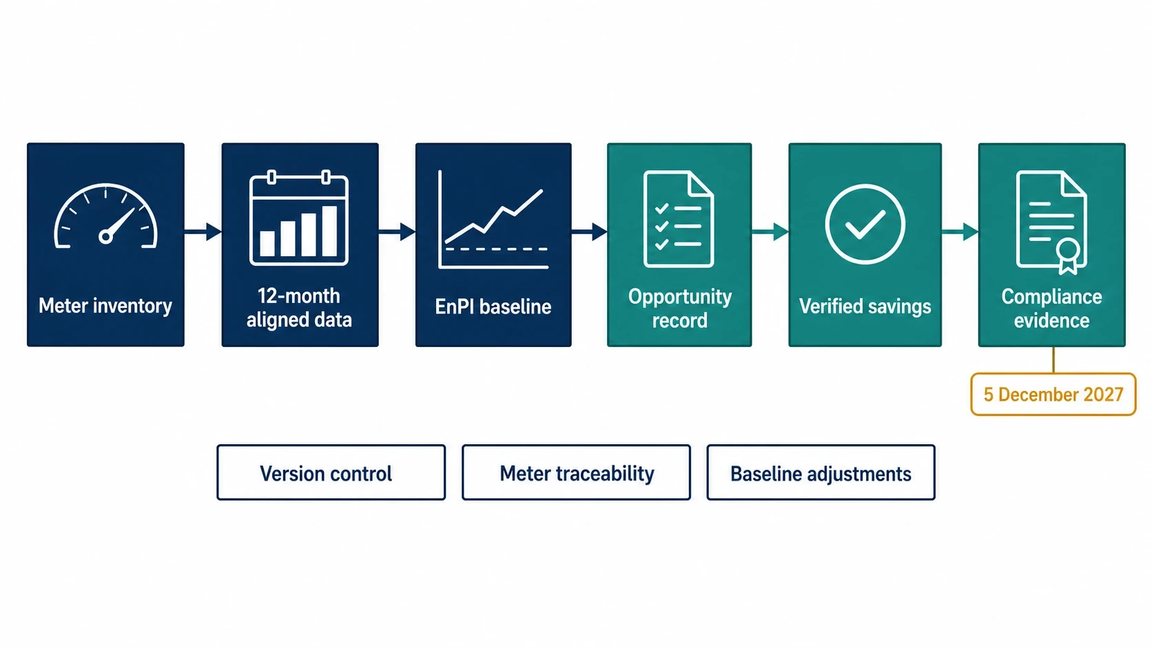
The Phase 4 notification deadline is 5 December 2027. The ESOS report must include estimated savings achieved during the compliance period, details of implemented measures and the energy saving associated with each measure in kWh. It must also categorise the savings and review relevant commitments from the preceding action plan.
A plant-wide benchmarking programme can support this evidence through:
- Meter inventories and documented boundaries
- Twelve months of aligned utility and production data
- Defined EnPIs and baseline methods
- Records of estimates and missing-data treatment
- Opportunity assessments and implementation dates
- M&V plans
- Post-implementation results
- Reasons for projects that were deferred or rejected
The evidence pack should retain the data and methods behind reported calculations. Benchmarking records therefore need version control, meter traceability and documented baseline adjustments, as well as dashboard outputs.
Applying Omni Vision to plant-wide benchmarking
Omni Vision combines utility metering with production-linked KPI reporting across electricity, gas, water, steam, compressed air and oil. Its hierarchy can connect the site total to departments, utility systems, production lines and selected equipment.
The benchmarking design should begin with decisions. A food manufacturer may need electricity per tonne, refrigeration consumption by production state and water per cleaning cycle. A batch chemical plant may obtain more value from gas per batch, steam per product grade and non-production electrical demand.
Within Omni Vision, a meaningful exception alert should compare measured consumption with an expected value derived from matched operating conditions. The alert should identify the meter, interval, predicted consumption, actual consumption, residual and threshold breached. Forecasting should apply the same documented consumption relationships to planned throughput and operating conditions, producing an expected utility requirement for teams to review against subsequent readings. Operators or building-management systems can then act on validated recommendations during approved change windows.
EnerTherm Engineering publishes an 8 to 16-week deployment window for Omni Vision. The site survey should use that period to settle boundaries, production variables, data ownership and initial M&V priorities. Meter installation alone does not create a defensible benchmark. Data validation, operating-state classification and agreement on the baseline complete the measurement system.
The management cycle moves from measuring utility use and normalising it against production to investigating material deviations, pricing the avoidable portion, approving an intervention and verifying the outcome.
This article reflects the independent analysis and editorial opinion of EnerTherm Engineering. Product names, trademarks, and brands mentioned belong to their respective owners. EnerTherm Engineering is not affiliated with, endorsed by, or a licensee of any third-party software or product mentioned unless explicitly stated.

Technical Manager — EnerTherm Engineering
John Naranjo is Technical Manager at EnerTherm Engineering, bringing specialist expertise in chemical and environmental engineering. He recently led the implementation of Omni Vision, EnerTherm's real-time energy and utility monitoring platform. He holds an MSc in Environmental Engineering from the University of Huelva and a BSc in Chemical Engineering, with memberships in both the Energy Institute and IChemE.
