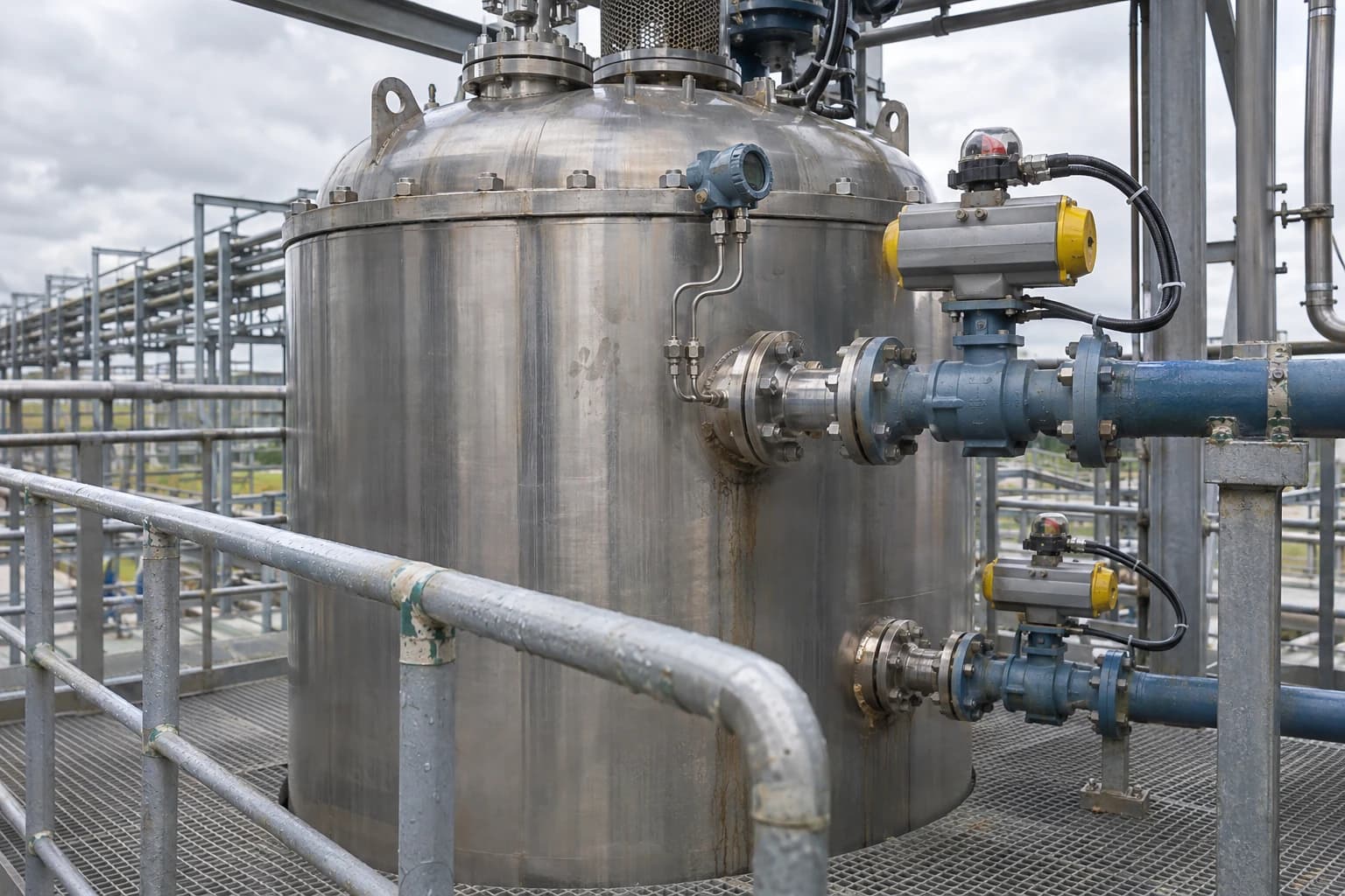
Dynamic Process Simulation Calculates Process Safety Time
Transient models validate SIS response against BS EN 61508 and BS EN/IEC 61511.
Dynamic process simulation is the time-dependent modelling of mass, energy, momentum and control responses in a process. It calculates how long a plant can tolerate a fault before it reaches an unsafe condition.
That interval is Process Safety Time, or PST. For a high-temperature reactor, it may run from loss of cooling to a runaway temperature. For a distillation column, it may run from a reflux failure to flooding or overpressure. For a separator, it may run from compressor trip to pressure reaching a vessel limit.
Steady-state models cannot calculate that interval. They resolve an operating point. Dynamic process simulation resolves the route between operating points, including equipment holdup, heat transfer, reaction kinetics, valve movement, controller action and the changing thermodynamic state of the inventory.
For principal process engineers and control systems design leads, PST links a process hazard to a timed safety function. It determines whether a sensor, logic solver and final element can move the plant to its defined safe state before the hazardous consequence develops.
What is Process Safety Time in dynamic process simulation?
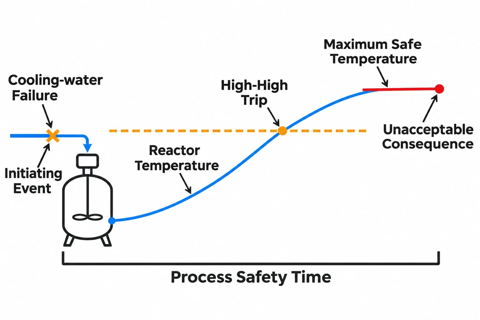
Process Safety Time is the maximum elapsed time between the onset of a hazardous deviation and the point at which the process reaches an unacceptable consequence. The consequence may be a pressure limit, temperature limit, loss of containment, unstable reaction rate, dry-running pump condition or another documented hazard endpoint.
The timer starts at the initiating event, not at the alarm setpoint or safety-instrumented-function trip setpoint. A cooling-water failure might begin at time zero, while a reactor high-high temperature trip occurs only after the vessel inventory has absorbed heat and the temperature has climbed to its trip setting.
Why the endpoint must be explicit
A credible PST calculation needs an unambiguous endpoint. “Thermal runaway” is too broad for a safety requirements specification. A useful endpoint can be one of the following:
- Reactor temperature reaches the established maximum safe operating temperature.
- Vessel pressure reaches maximum allowable working pressure.
- Reaction rate enters the identified accelerating region.
- A column differential pressure reaches the flooding criterion.
- A liquid level reaches the point at which gas carry-over or liquid carry-over creates a defined hazard.
- A relief valve lifts, where the study objective is to avoid loss of normal containment or excessive flare loading.
The selected endpoint must reflect the hazard assessment. It should not be selected because it is easy to simulate or matches an available transmitter range.
PST is a process property, not a control-system setting
PST belongs to the process and its physical response. It changes with reactor inventory, feed composition, catalyst condition, utility temperature, vessel pressure, heat-transfer area, operating mode and the scenario being examined.
A reactor can therefore have different PST values for loss of agitation, cooling-water loss, excessive reactant charge, high initiator concentration and blocked outlet. A single generic PST for the entire unit can hide the limiting case.
The simulation must distinguish between normal control action and independent protection. A basic process control system may arrest a minor disturbance. A safety instrumented system must still perform when the initiating failure disables, bypasses or overwhelms the control loop assumed in the model.

Map every energy and material flow in your process with detailed heat and mass balance calculations — the foundation for any optimisation or design project.
Why steady-state heat and mass balances cannot establish PST
A steady-state heat and mass balance establishes compositions, duties, temperatures, pressures, utility loads and expected operating envelopes. Dynamic process simulation then adds accumulation and time.
Equipment holdup sets the clock
Liquid volume in a reactor, drum or column sump stores material and sensible heat. Vapour volume stores compressible inventory. Metal walls, coils and exchanger shells add thermal inertia. These properties dictate how fast a deviation turns into a hazard.
Consider a jacketed batch reactor. Loss of cooling may initially produce a gradual temperature rise because the vessel wall and liquid inventory absorb energy. As the reaction accelerates with temperature, heat generation can exceed the remaining heat-removal capacity. The temperature trajectory then steepens sharply. A steady-state model can indicate an unfavourable energy balance. A dynamic model identifies the time available before the selected hazard endpoint.
Thermodynamics and kinetics must remain credible outside normal operation
PST often depends on conditions outside the usual design case. A pressure fall can cause flashing and lower vessel temperature. A pressure rise can change vapour-liquid equilibrium and vapour generation. A feed transition can alter reaction rate, density, heat capacity and condenser load.
The model requires an appropriate property method, representative reaction kinetics, heat-transfer correlations and validated equipment geometry. An impressive trend from an unvalidated model has no safety value.
Where reaction kinetics are uncertain, engineers should test credible bounds. The limiting PST may emerge from a conservative kinetic case, reduced cooling coefficient, fouled exchanger, high reactant concentration or low initial inventory. Sensitivity analysis turns uncertainty into an auditable design decision.
Control loops change the transient trajectory
A dynamic model should include the control loops available during the scenario, with realistic controller mode, tuning, output limits, valve characteristics, deadband and actuator travel time.
This matters during:
- Startup, when inventories and temperatures move through unstable regions.
- Shutdown, when heat input, reflux, agitation or circulation may be removed in sequence.
- Feedstock changeover, when composition control and heat-release behaviour can move together.
- Compressor trip, when anti-surge action, recycle capacity and downstream pressure interact.
- Emergency depressurisation, when pressure, temperature, phase behaviour and flare-header backpressure develop simultaneously.
A controller that works around the steady-state operating point can behave poorly during a large transient. Integral wind-up, saturated valves and delayed temperature response can create a false sense of available time.
How a dynamic process simulation calculates PST
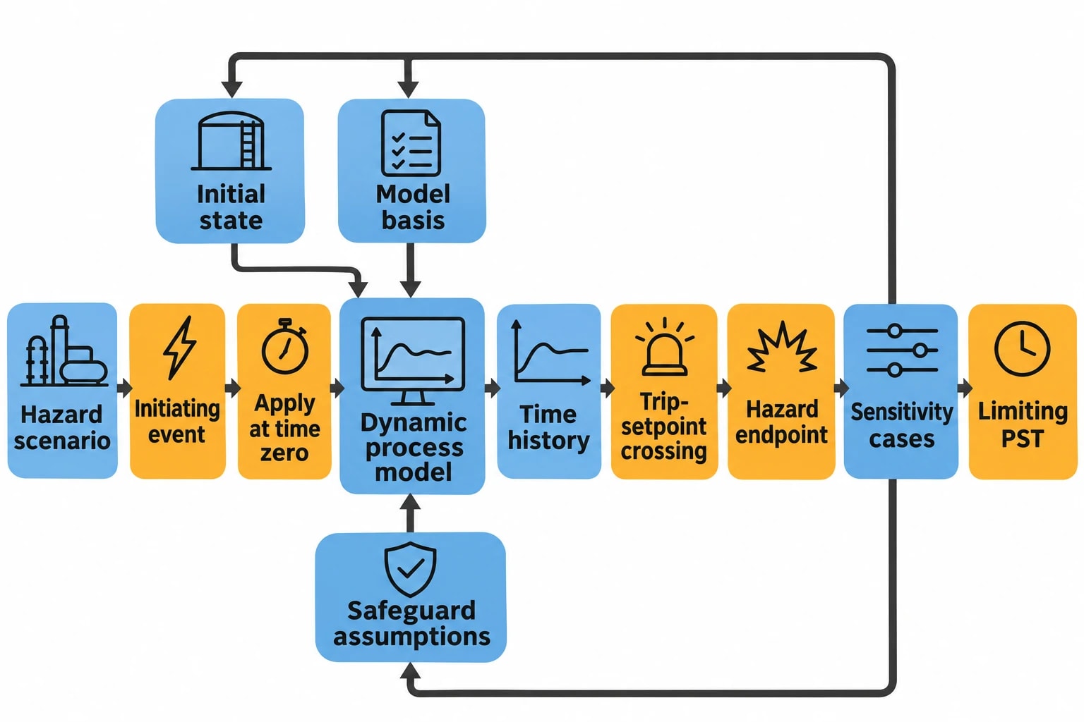
The calculation is a controlled scenario study, not a single simulator run. Its value lies in traceability from hazard to model assumptions, transient result and safety requirement.
1. Define the initiating event and hazardous consequence
Start with the HAZOP, layer-of-protection analysis, process hazard analysis or operating-history evidence. State the initiating event precisely. “Cooling failure” must distinguish between total cooling-water loss, reduced flow, loss of refrigerant, failed cooling-water control valve or heat-transfer impairment.
State the consequence and threshold with equal precision. For example: “reactor pressure reaches the vessel’s maximum allowable working pressure” or “reactor bulk temperature reaches the approved maximum safe operating temperature”.
2. Establish the initial operating state
The model must start from a credible operating condition. This includes plant throughput, composition, pressure, temperature, liquid levels, equipment duty, valve position and controller mode.
A safety study should not rely only on nominal design conditions. The team should identify operating states that plausibly reduce available time. A high reaction concentration, hot summer cooling-water supply, high catalyst activity or high liquid level can change the result materially.
3. Represent the physical inventory and safety barriers
Model the vessels, piping sections and heat exchangers that materially affect the transient. Include appropriate upstream and downstream boundary conditions. A relief calculation may require the connected pressure network rather than an isolated vessel because header backpressure can alter discharge behaviour.
Represent the safeguards included in the scenario:
- Basic process control loops.
- Alarms and operator actions, where the response time is justified.
- Safety instrumented functions.
- Emergency shutdown valves.
- Blowdown valves.
- Pressure-relief devices and flare connections.
- Agitation, recirculation and utility systems where their failure or availability changes the consequence.
Each safeguard needs an independent basis. A model should not credit a control valve that fails in the same mode as the initiating event.
4. Apply the fault and measure the time to the endpoint
Apply the initiating deviation at time zero. Record the time history of the key variables and the time at which the selected hazard endpoint occurs. That elapsed time is the calculated PST for that scenario and initial condition.
The study should also identify the trip-setpoint crossing time. This separates process development from safety-system response. If a temperature trip activates close to the hazard endpoint, the safety function may have little usable response margin even if the final temperature trend appears controllable.
5. Test sensitivity and identify the limiting case
The reported PST should be the limiting credible value, not an average result. Vary uncertain or operationally significant inputs and document the case that produces the shortest time to the defined consequence.
A concise calculation record should include the following.
| Item | Evidence required |
|---|---|
| Hazard scenario | Initiating event, causes and consequence from the hazard study |
| Process endpoint | Defined pressure, temperature, level or other safety threshold |
| Initial state | Operating case, inventory, composition, utility conditions and controller modes |
| Model basis | Property method, kinetic basis, equipment data and boundary conditions |
| Safeguard assumptions | Credited loops, trips, alarms, valves and response times |
| PST result | Time from initiating event to endpoint for each scenario |
| Sensitivity cases | Inputs tested and the identified limiting result |
| Validation status | Comparison against plant data, tests, vendor data or accepted design information |
Map every energy and material flow in your process with detailed heat and mass balance calculations — the foundation for any optimisation or design project.
Turning PST into a safety instrumented system requirement
The safety requirements specification should use the PST result to establish the maximum permitted response time for the safety instrumented function.
HSE identifies BS EN 61511 as the benchmark standard for functional safety management in process industries. The standard covers the specification, design, installation, operation and maintenance of safety instrumented systems. BS EN 61508 provides the broader functional-safety framework for electrical, electronic and programmable electronic safety-related systems.
Account for the whole safety-function response
The relevant response time is not the logic solver scan time. It includes the full path from detection of the hazardous condition to completed final action:
- Process transmitter sensing and signal processing.
- Input processing and safety logic execution.
- Output action and actuator energisation.
- Final-element movement, such as valve closure or pump trip.
- Process response after the final element reaches its required position.
Large shutdown valves can dominate this time budget. A valve may close slowly because of actuator sizing, hydraulic restriction, stroking characteristics, process differential pressure or fail-safe arrangement. The dynamic model should represent the physical effect of that movement rather than treating closure as instantaneous.
Many organisations apply a 2:1 design margin, setting maximum safety-function response time at no more than half of the calculated PST. That margin allows for modelling uncertainty, instrument response variation, process variability and ageing of final elements. It should be documented as an engineering requirement for the application, rather than presented as a substitute for the lifecycle requirements of BS EN 61511.
Separate BPCS and SIS claims
The basic process control system normally manages production and ordinary disturbances. The SIS provides a defined risk-reduction layer when a hazardous condition develops. HSE guidance notes that a safety instrumented system typically comprises sensors, logic functions and final elements that bring the process to a safe state.
A dynamic study should therefore test at least two cases where appropriate:
- The control system responds as intended and prevents escalation.
- The control action is unavailable, ineffective or insufficient, requiring SIS action.
This separation exposes whether the selected trip setpoint and final-element action remain adequate under the failures that matter.
Thermal runaway, overpressure and emergency relief scenarios
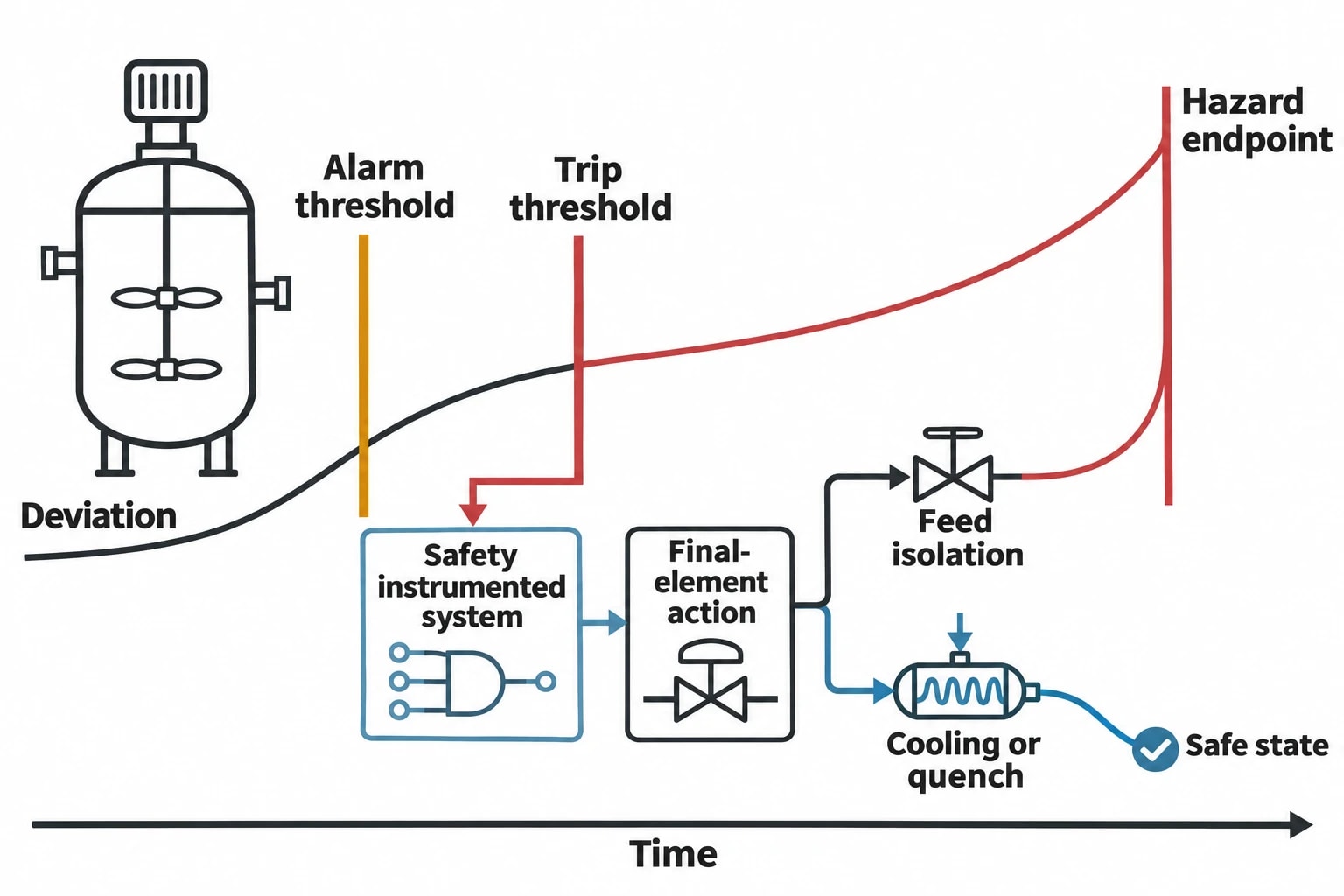
Dynamic process simulation is particularly valuable where time-dependent interactions invalidate simple conservative assumptions or create unnecessary oversizing.
Thermal excursions in reactive systems
For exothermic reactors, model the reaction heat, cooling system, vessel heat capacity, agitation state, feed timing and any quench or inhibitor addition. The key output is not only peak temperature. It is the time sequence: onset of deviation, alarm threshold, trip threshold, final-element action and approach to the hazard endpoint.
A realistic case may show that stopping feed stabilises the process. Another may show that residual reactant and stored heat continue the excursion after feed isolation. That distinction determines whether the safety function must also initiate cooling, quench, venting, agitation or emergency depressurisation.
Pressure-relief and flare-network studies
ISO 23251:2019 addresses pressure-relieving and vapour-depressuring systems for petroleum, petrochemical and natural-gas industries. Relief loads, disposal piping, flare systems and vent stacks form an interacting pressure system.
For complex events, a dynamic model can calculate time-varying relief flow, composition, vapour fraction, vessel pressure, blowdown temperature and header backpressure. These variables affect whether a pressure-relief device performs as assumed and whether a flare network can manage coincident discharges.
Commercial simulation packages including Aspen HYSYS Dynamics and CC-DYNAMICS provide dynamic modelling capabilities for startup, shutdown, relief and depressurisation studies. Their output remains dependent on the thermodynamic method, physical model, equipment data and scenario assumptions entered by the engineering team.
Machine trips and utility failures
A compressor trip can propagate upstream and downstream through recycle action, separator pressure, fired-heater feed, flare load and liquid-level control. A total power loss can remove several safeguards at once. Dynamic studies should apply the actual trip sequence, including available emergency power, valve fail positions, inertial run-down and utility persistence.
The limiting scenario may not be the largest initial pressure rise. It may be the case where a delayed secondary effect reaches a vulnerable vessel after a control valve saturates or a pressure network develops backpressure.
Building a defensible dynamic simulation workflow
A useful PST result must survive review by process safety, controls, operations and project engineering. That requires a disciplined heat and mass balance workflow.
Build from a validated steady-state foundation
EnerTherm Engineering’s Heat and Mass Balance methodology begins with process documentation, operating data and site-specific evidence before forming a validated process-flow basis. For dynamic work, that baseline should include P&IDs, stream data, equipment geometry, control narratives, alarm and trip setpoints, valve data, historical trends and operating procedures.
The steady-state model establishes the mass and energy balance. The dynamic model adds vessel holdup, heat-transfer surfaces, pressure-flow relationships, control configuration and event logic.
Validate against behaviour, not only normal operation
A model matched only to a normal operating point may still misrepresent a trip. Validation should compare predicted behaviour with available plant responses, startup data, step tests, shutdown records or commissioned equipment performance.
Reviewers should challenge:
- Whether vessel volumes and liquid levels are correct.
- Whether heat-transfer coefficients reflect fouling and operating condition.
- Whether control valves use credible characteristics and travel times.
- Whether relief or blowdown paths include relevant downstream pressure effects.
- Whether the selected reaction model reflects the hazardous chemistry.
- Whether credited safeguards remain independent of the initiating cause.
Deliver an engineering decision, not a trend plot
The final deliverable should state the limiting scenario, calculated PST, required maximum safety-function response time, trip-setpoint basis, assumed final-element action and remaining uncertainty. It should also identify design changes that increase available time, such as reducing inventory, increasing cooling duty, revising trip setpoints, improving valve stroking time or separating dependent safeguards.
That result can then enter the safety requirements specification, cause-and-effect chart, control narrative, relief study and commissioning test plan. Dynamic process simulation turns the transient into an engineering basis that can be checked before plant startup and maintained through later modifications.
This article reflects the independent analysis and editorial opinion of EnerTherm Engineering. Product names, trademarks, and brands mentioned belong to their respective owners. EnerTherm Engineering is not affiliated with, endorsed by, or a licensee of any third-party software or product mentioned unless explicitly stated.

Simulation Engineer — EnerTherm Engineering
Rajesh Sekar is a Simulation Engineer at EnerTherm Engineering, specialising in computational fluid dynamics (CFD), finite element analysis (FEA), and thermal process simulation. He holds a degree from Cranfield University and brings extensive experience in simulation-based product development from the automotive, aerospace, and energy sectors.
