
Pinch Analysis Methodology: Two Routes to Heat Targets
How Problem Tables and Composite Curves set minimum utility targets
A pinch analysis methodology is a thermodynamic method that calculates the minimum heating and cooling utilities a process requires and uses those targets to guide heat recovery and heat exchanger network design.
A refinery crude preheat train, a pharmaceutical solvent-recovery unit and a food evaporation system face the same practical question: how much heat can streams that need cooling transfer to streams that need heating before the site draws additional steam, fuel, thermal oil, cooling water or refrigeration?
Pinch analysis answers this question before exchanger duties, surface areas and network topology are fixed. It takes a reconciled heat and mass balance, applies a selected minimum approach temperature, ΔTmin, and identifies the maximum achievable process-to-process heat recovery. The resulting targets establish the minimum hot utility, minimum cold utility and pinch temperature.
Ian C. Kemp’s Pinch Analysis and Process Integration: A User Guide on Process Integration for the Efficient Use of Energy, second edition, remains a principal reference for the discipline. It sets out two complementary routes to energy targets: Composite Curves, the graphical route, and the Problem Table Method, the numerical route. Both begin with the same stream data and should produce the same utility targets.
Why pinch analysis methodology starts with targets
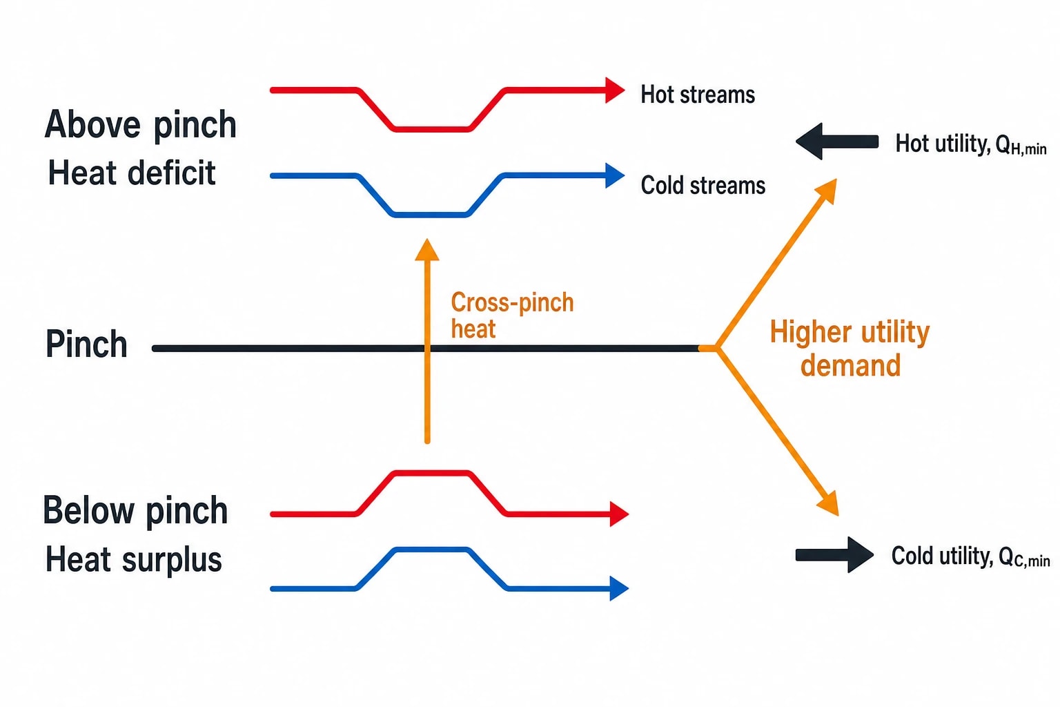
Process integration and pinch analysis separate energy targeting from heat exchanger network synthesis. This gives engineering teams a benchmark before they commit to equipment changes.
A plant may add several heat exchangers and still fall well short of its thermodynamic potential. An existing network can conceal poor temperature matching, misplaced utility use, bypassed recovery, fouling or process conditions that create unnecessary heating or cooling loads. A utility target exposes the gap.
The method combines process streams into two groups:
- Hot streams release heat as they cool, condense or undergo another exothermic duty.
- Cold streams require heat as they warm, evaporate or undergo another endothermic duty.
The analysis establishes three linked results:
- Minimum hot utility, QH,min, such as steam, fired-heater duty or thermal oil.
- Minimum cold utility, QC,min, such as cooling water, air cooling or refrigeration.
- Maximum heat recovery, the greatest internal process-to-process recovery consistent with the chosen ΔTmin.
The pinch is a calculated temperature constraint, not plant equipment. Above the pinch, the process has a heat deficit. Below it, the process has a heat surplus. Heat transferred across this boundary raises hot and cold utility demand by the same amount.
The pinch is therefore a design discipline as well as an energy target. It directs attention to heat quality, not simply quantity. A large duty at 60 °C may be valuable for feed preheating or hot-water production, yet cannot directly replace a reboiler duty at 170 °C.

Map every energy and material flow in your process with detailed heat and mass balance calculations — the foundation for any optimisation or design project.
Build a sound heat and mass balance first
Define the operating case
A pinch calculation represents a specific operating condition, so the stream data needs a clear basis.
For a continuous chemical plant, that basis may be a stated throughput, feed composition, product slate and utility condition. In oil refining, crude characteristics, unit severity and seasonal cooling-water conditions can materially change available recovery. Pharmaceutical batch operations often require a time-dependent study because heat sources and demands may not occur simultaneously.
A grassroots project needs design cases, credible turndown and anticipated utility conditions. A retrofit needs representative plant cases alongside cases that define operating limits. A single annual average can conceal the temperature-driving-force problems that appear at lower throughput or during seasonal changes.
Extract streams with traceable data
Each candidate stream needs enough detail to establish its temperature interval, heat duty and operating constraints. The stream register should remain traceable to current process flow diagrams, P&IDs, laboratory data, historian records and utility metres.
| Stream field | Purpose in the pinch study |
|---|---|
| Stream identity and service | Connects the calculation to plant equipment and PFD stream tables |
| Hot or cold classification | Identifies whether the stream releases or requires heat |
| Supply and target temperature | Defines the available temperature interval |
| Heat-capacity flow rate | Determines sensible heat duty over that interval |
| Latent or reaction duty | Captures condensation, evaporation, boiling or reaction heat |
| Pressure and phase behaviour | Supports correct enthalpy and temperature treatment |
| Operating availability | Confirms whether source and sink operate at the same time |
| Fouling, contamination and materials limits | Defines feasible heat-exchanger matches |
Engineers should account for phase change explicitly. Treating a condensing vapour as a simple sensible stream can distort both the Composite Curves and the utility target. The same applies to boiling, evaporation, crystallisation, melting and reaction duties where process enthalpy changes sharply over a narrow temperature range.
Reconcile the data before targeting
The total heating and cooling duties in the stream table should reconcile with fuel consumption, steam generation, cooling-water loads, refrigeration duty and known process heat losses. A discrepancy needs investigation before the calculation progresses.
Common sources of error include incorrect steam pressure, unrecorded condensate-return conditions, missing latent heat, changing production rate, unmetered vent losses, heat tracing, incorrect heat-exchanger bypass positions and out-of-date drawings. A misplaced target temperature can create a substantial false recovery opportunity.
The study record should document the data source, date range, throughput basis, heat-capacity assumptions, utility conditions, phase treatment, excluded streams and operating constraints. This creates an auditable engineering baseline for later process changes.
Choose the minimum approach temperature
Shift temperatures by half of ΔTmin
Pinch analysis uses shifted temperatures to embed the selected ΔTmin in the target calculation. Hot-stream temperatures shift down by half of ΔTmin. Cold-stream temperatures shift up by half of ΔTmin.
For a selected ΔTmin of 20 °C, hot-stream temperatures shift down by 10 °C and cold-stream temperatures shift up by 10 °C. The process itself does not change temperature. The shifted scale allows the Composite Curves or heat cascade to identify a pinch while maintaining the intended real temperature difference between hot and cold streams.
This convention produces two actual pinch temperatures when the result is converted back. The hot-side pinch temperature lies ΔTmin above the cold-side pinch temperature.
Select ΔTmin as an economic design choice
ΔTmin governs the trade-off between energy consumption and heat-exchanger capital cost. A smaller approach generally increases heat recovery but also increases required heat-exchanger area and may introduce more complex network arrangements. A larger approach reduces heat-exchanger area while increasing utility consumption.
The appropriate value depends on:
- Stream fouling and cleaning intervals.
- Fluid viscosity and heat-transfer coefficients.
- Phase change and condensing services.
- Allowable pressure drop.
- Materials selection and corrosion risk.
- Plot space and piping complexity.
- Utility price, fuel price and operating hours.
- Carbon-cost exposure and expected plant life.
A useful heat-integration study tests several ΔTmin values. For each value, the team calculates hot and cold utility targets and estimates heat-exchanger area and capital cost. This cost-targeting exercise is commonly called supertargeting.
A single default ΔTmin may be acceptable for an early screen. Detailed design often needs different practical approach temperatures for services with sharply different heat-transfer behaviour. Clean liquid-liquid exchange, viscous product streams, gases, slurries and condensing steam should not receive identical assumptions without engineering justification.
Route one: Composite Curves for graphical heat targets
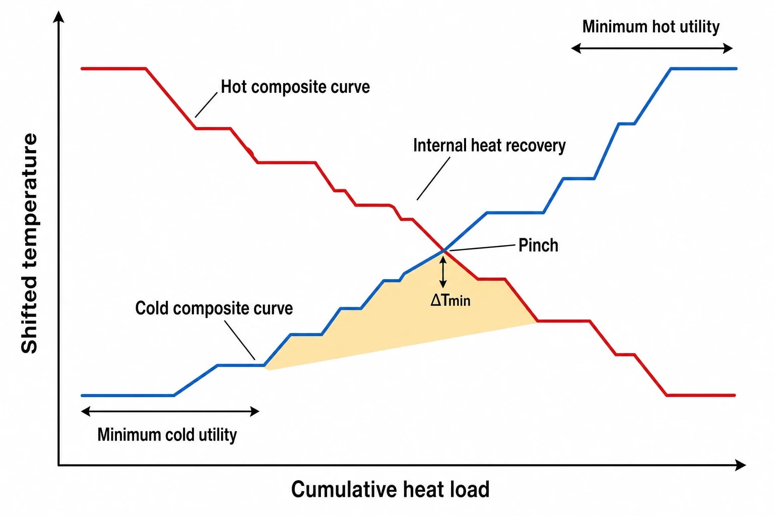
What Composite Curves represent
Composite Curves plot cumulative heat load against temperature. The hot composite curve combines heat released by hot process streams across their temperature ranges. The cold composite curve combines heat required by cold process streams.
The analyst positions the curves until they touch at the pinch on the shifted temperature scale, representing the selected ΔTmin in real temperatures. The horizontal separation at the hot end gives the minimum hot utility target. The separation at the cold end gives the minimum cold utility target.
The graphical result communicates several engineering features quickly:
- The overlap indicates the potential for internal heat recovery.
- The high-temperature gap identifies the requirement for hot utility.
- The low-temperature gap identifies the requirement for cold utility.
- Curve slopes reflect the combined heat-capacity flow rate of streams active in each temperature range.
- A steep section or discontinuity can reveal stream starts, stream ends or phase-change duties.
Read temperature quality as well as duty
Composite Curves make a frequent error visible. Total hot-stream duty may appear sufficient to meet total cold-stream duty, while the available heat sits at temperatures too low for the process demand.
Consider a chemical process with substantial warm effluent at 80 °C and a distillation reboiler requiring heat above 150 °C. The warm effluent may reduce cooling demand or preheat incoming feed, but cannot satisfy the reboiler directly. The curves show where that temperature mismatch occurs.
Composite Curves turn a large stream table into a temperature-duty picture that can guide discussions on feed preheating, utility levels, waste-heat recovery and process changes.
Use the graphical result as a check
Composite Curves are a targeting method, not a substitute for a validated stream register. Their value depends on correct stream enthalpies, phase treatment and ΔTmin assumptions. A chart generated from poor data can look convincing while setting an unreliable target.
The graphical result should be checked against the Problem Table Method. Agreement between the two provides confidence that the stream intervals, temperature shifts and utility targets have been handled consistently.

Map every energy and material flow in your process with detailed heat and mass balance calculations — the foundation for any optimisation or design project.
Route two: the Problem Table Method
Build the temperature intervals
The Problem Table Method, also called the heat cascade, converts the stream problem into a numerical sequence. It begins with the shifted supply and target temperatures for each process stream.
The analyst then:
- Lists the unique shifted temperatures in descending order.
- Defines the temperature intervals between adjacent values.
- Identifies hot and cold streams active within each interval.
- Calculates the net heat-capacity flow rate for each interval.
- Determines the interval heat surplus or deficit.
- Cascades the residual heat from the highest shifted interval to the lowest.
The interval calculation is based on the combined heat-capacity flow rates of the active hot and cold streams and the interval temperature span. The method handles a large stream set more clearly than hand-drawn curves and creates an auditable calculation trail.
Find QH,min and QC,min
The first cascade starts with zero heat at the highest shifted temperature. A negative residual means the process lacks heat at that temperature level. The most negative residual determines the minimum hot utility required to eliminate every negative value.
The analyst adds that duty at the top of the cascade and repeats the calculation. The final residual at the lowest interval is then the minimum cold utility target, QC,min. The interval where the adjusted residual reaches zero identifies the pinch.
This numerical route explains why a process with balanced total hot and cold duties can still require both heating and cooling utilities. Heating and cooling needs occur at different temperature levels. A site cannot use surplus low-grade heat to meet a higher-temperature deficit without an appropriate utility or technology that raises its temperature.
Why the numerical route matters in practice
The Problem Table Method works well in spreadsheets, process-simulation exports and sensitivity studies across several ΔTmin values. It allows an engineer to inspect each temperature interval, identify a problematic stream combination and repeat the target after a process change.
Pinch analysis software can calculate intervals, draw curves and produce network concepts quickly. Thermal design teams still need to assess stream selection, control implications, phase behaviour, heat-exchanger fouling, pressure drop and plant access. The software performs the arithmetic; engineering judgement determines whether an apparent recovery opportunity is operable and economically justified.
Apply targets to heat exchanger network synthesis
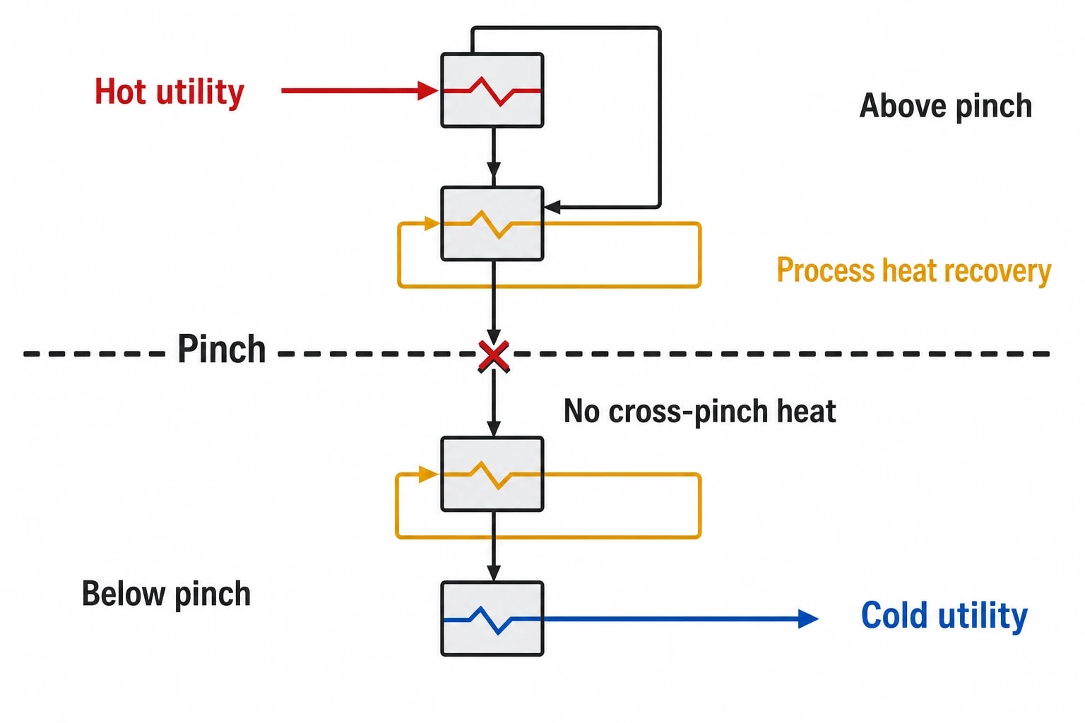
Follow the pinch design rules
Once the team has set energy targets, heat exchanger network synthesis can begin. At the minimum utility target, the initial network should follow three established rules:
- Do not transfer heat across the pinch.
- Do not use cold utility above the pinch.
- Do not use hot utility below the pinch.
Cross-pinch exchange increases hot and cold utility requirements by the same duty. Cold utility above the pinch removes heat from a region with a heat deficit. Hot utility below the pinch adds heat to a region with a heat surplus.
These rules establish the starting point for heat exchanger network synthesis. A real project may accept a utility penalty to reduce capital cost, avoid an unsafe match, simplify control or work around fixed equipment. The business case should quantify that penalty rather than treat it as an unexplained design feature.
Use the Grand Composite Curve for utilities
The Grand Composite Curve represents the net heat cascade against shifted temperature. It shows where the process has a heat deficit or surplus after maximum process heat recovery.
This provides a direct way to examine utility temperature levels. A Grand Composite Curve can help assess the fit of high-pressure steam, medium-pressure steam, hot water, cooling water, refrigeration or a heat pump to the remaining process requirement.
For example, a refinery study may use the curve to examine the relationship between crude preheat, fired-heater demand and steam levels. A chemical site may focus on distillation reboilers and condenser duties. Food and beverage facilities may assess the temperature relationship between evaporation, pasteurisation and cleaning systems.
The curve does not select the utility automatically. It provides a temperature-based basis for evaluating utility integration against actual duty, operating and capital constraints.
Grassroots and retrofit studies take different routes
Grassroots design
A grassroots plant allows designers to develop process conditions, utility levels, plot arrangement and heat exchanger network topology together. Pinch targets should influence the flowsheet before equipment specifications become fixed.
This makes it possible to reduce heating and cooling requirements through process design as well as heat-exchanger matching. Engineers can consider feed conditioning, separation pressure, utility generation and heat-exchanger placement while the project retains flexibility.
Design cases still need attention. A network that reaches its target at full throughput may create poor temperature driving forces at turndown or under seasonal cooling-water conditions. The final design should test credible operating cases and include bypass, control and maintenance requirements.
Retrofit applications
Retrofit applications begin with an installed heat exchanger network and its constraints. Existing heat-exchanger area, piping routes, pressure drop, plot space, fouling history, shutdown windows and control loops shape the achievable project.
The gap between current utility use and the pinch target is a screening measure, not an automatic savings commitment. Some of that gap may be technically inaccessible or uneconomic to recover.
Typical retrofit opportunities include heat-exchanger cleaning, bypass removal, duty reallocation, revised utility temperatures, restored area, feed-effluent exchange, heat-exchanger additions and phased repiping. Each option requires testing against temperature feasibility, recoverable duty, installation complexity, production risk and maintenance access.
A match that performs well at high throughput can fail at lower rates because the available driving force decreases. Multiple operating cases are therefore central to retrofit targeting.
Turn heat targets into an engineering decision
Pinch analysis has value when the target calculation leads to a disciplined list of actions. The final package should link the stream table, Composite Curves, Problem Table, Grand Composite Curve, heat and mass balance and current utility use.
Each proposed heat-recovery measure should state:
- The source and sink streams.
- Available duty and temperature range.
- Selected ΔTmin and expected approach temperature.
- Expected effect on hot and cold utility demand.
- Required heat-exchanger area or equipment changes.
- Fouling, contamination, pressure-drop and control constraints.
- Operating cases where the match remains feasible.
- Assumptions requiring plant measurement or testing.
Composite Curves provide the graphical explanation, while the Problem Table Method provides the numerical audit trail. Together they establish defensible heat targets before equipment design begins, giving process engineers a structured route from a reconciled heat and mass balance to practical thermal efficiency optimisation.
This article reflects the independent analysis and editorial opinion of EnerTherm Engineering. Product names, trademarks, and brands mentioned belong to their respective owners. EnerTherm Engineering is not affiliated with, endorsed by, or a licensee of any third-party software or product mentioned unless explicitly stated.

Simulation Engineer — EnerTherm Engineering
Rajesh Sekar is a Simulation Engineer at EnerTherm Engineering, specialising in computational fluid dynamics (CFD), finite element analysis (FEA), and thermal process simulation. He holds a degree from Cranfield University and brings extensive experience in simulation-based product development from the automotive, aerospace, and energy sectors.
